No-Regret Learning in Blotto Game (ongoing)

Summary

The work based on the paper

Introduction

A Colonel Blotto game is a type of two-person constant-sum game in which the players are tasked to simultaneously distribute limited resources over several battlefields.

Blotto game has fruitful applications in competitive sports. In multi-players sports (such as soccer, basketball, dota), a team need to distribute players into different positions to attack and defense in either right-side or left-side. In single-player sports (such as tennis, badminton), Players need to choose their focus in midfield and backcourts.

Blotto Game can be also used as a metaphor for electoral competition, with two political parties devoting money or resources to attract the support of a fixed number of voters.

No-Regret learning algorithm is a learning scheme that player will choose actions that would have better performance in the past.

A brief talk to the Blotto Game

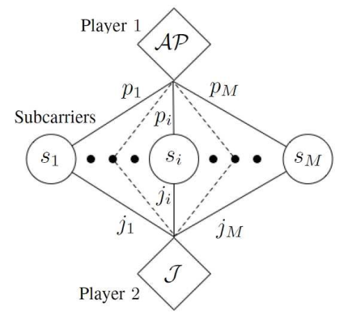
Blotto game is a two-person constant sum game, which two players \(P_1,P_2\) have limited resources \(S_1,S_2\) . Players will distribute the resources into several containers (battlefields) \(M\), where \(M>min(S_1,S_2)\). Players are allowed to distribute nothing in a container. For each container, the player who devotes most will claim a win on this container. If two players devote the same amount of resources, no one can have a win on this container but a draw. For each round, the player who wins more containers wins this round, otherwise, there is a draw this round.

https://ieeexplore.ieee.org/document/7841922

Discrete Blotto Game

In the discrete Blotto Game, the resources allocated to each battlefield must be an integer, which suggests the space of actions is finite. Moreover, the opponent’s action is also finite. Therefore, the space of action profiles is finite, and we can use a matrix to represent all the action profiles by letting rows indicate actions from the first player and columns indicating actions from the second player.

In the following discussion, we use an example about the small game that has 5 indivisible resources and 3 containers. For example, we can use a triple array to describe a player’s action of distribution of resources. (E.g.\([1,2,2]\), \([4,0,1]\),\([0,2,3]\))

Consider in a round, Player A chooses the action \([1,2,2]\) while Player B chooses the action \([3,0,2]\), then Player A win the second container (battlefield) and Player B wins the first container (battlefield) and two players have a draw on the third container (battlefield). Therefore, in this round, both player has one win one loss, and one draw hence the draw in this round.

For example, in the \((S = S_1 = S_2 = 5,M = 3)\) game, a player can in general have 5 kinds of action of allocation. This is shown by the fact that there are 5 ways, to sum up to 5 by 3 natural numbers, which are 5 = (5 + 0 + 0) = (4 + 1 + 0) = (3 + 2 + 0) = (3 + 1 + 1) = (2 + 2 + 1). In each allocation form, there are at most 6 ways of ordering. More specifically, [4, 1, 0] and [3, 2, 0] both has 6 ways, [3, 1, 1] and [2, 2, 1] and [5, 0, 0] both has 3 ways. Therefore, in each round, there are 21 actions each player can choose from. If we assign payoff 1 for a victory, -1 for a loss, and 0 for a draw, we can write all possible pairs of action of allocation into a n×n matrix, where n is the number of possibility of actions (n = 21 for (S = 5,N = 3)).

a payoff matrix P for the case (n = 21 for (S = 5,N = 3))

Each columns and rows represents an action from the following 21 actions list:

$$ \begin{array}{l} {\rm{[[0, 0, 5], [0, 1, 4], [0, 2, 3], [0, 3, 2], [0, 4, 1], }}\\ {\rm{[0, 5, 0], [1, 0, 4], [1, 1, 3], [1, 2, 2], [1, 3, 1], }}\\ {\rm{[1, 4, 0], [2, 0, 3], [2, 1, 2], [2, 2, 1], [2, 3, 0], }}\\ {\rm{[3, 0, 2], [3, 1, 1], [3, 2, 0], [4, 0, 1], [4, 1, 0], [5, 0, 0]]}} \end{array} $$

Consider the computation result that both players choose the mixed strategy \(v\)

\begin{equation} v = (0, 0, p, p, 0, 0, 0, p, 0, p, 0, p, 0, 0, p, p, p, p, 0, 0, 0); p=1/9 \end{equation}

Which represents all the \((3+2+0), (3+1+1)\) actions have a probability \(1/9\). Then we can have that

$$ Pv = \left( { p_2, p_1,0,0, p_1, p_2, p_1,0, p_1,0, p_1,0, p_1, p_1,0,0,0,0, p_1, p_1, p_2} \right) $$

where \(p_1= -1/9, p_2=-5/9\).

Notice that the maximal value in \(Pv\) is \(0\) which occur at the index \(i\) when \(v_i = 1/9\) which are \(i=3,4,8,10,12,15,16,17,18\). This suggests that the best response of \(v\) is the span of these base vectors.

$$ BR(v) = span\left\{ {e_i|{v_i} = p} \right\} $$

Therefore, \begin{equation} v \in BR_P(v) \end{equation} this suggests that the simulation result that two players choose mixed strategy \((v,v)\) is a Nash Equilibrium.

Continuum Blotto Game

In this section, We consider one of the simplest Blotto Game such that:

1. There are two battlefields.
2. Two players have different amount resources. (Blotto: 1, Enemy: E)
3. Two players can allocate any non-negative real number amount of resources to each battlefields.

The reason for the second condition is as follows. If two players have the same amount of resources, then we have a complete symmetric setting. Both players have the same space of action. While if player 1 wins a field, player 2 must win the other field, hence a draw. If two players allocate the same amount of resources on the two fields, it is also a draw. Therefore, for all action profiles, the result will be a draw and the payoffs for two players are both 0. This becomes a trivial game and no dynamics of learning between two players.

We can reduce the problem and consider the case when a player has 1 unit of troops and the second player has \(E<1\) unit of troops. Let say two players (Blotto and enemy) allocate \((b_1,b_2)\) and \((e_1,e_2)\) to two battlefields respectively. Notice that players are allowed to not allocate all the troops they have. Which are

$$ \begin{array}{l} {b_1},{b_2},{e_1},{e_2} \ge 0\\ {b_1} + {b_2} \le 1\\ {e_1} + {e_2} \le E \end{array} $$

Therefore we can use the following diagram to represent all the actions of two players.

Each point in the triangle represents an action. Then we can introduce the concept of payoff region about a point \((x_0,y_0)\) as following: \begin{equation} p(n;m)=p((x,y);({x_0},{y_0})) = {\mathop{\rm sgn}} \left( {x - {x_0}} \right) + {\mathop{\rm sgn}} \left( {y - {y_0}} \right) \end{equation} which can be illustrated by the following figure, which divide the plane into 4 region: win region, lose region, and two draw region.

We say that for a point \(m\),

$$ \begin{array}{l} WIN(m)=\{n| p(n;m) =2\}\\ LOSE(m)=\{n| p(n;m) =-2\}\\ DRAW(m)=\{n| p(n;m) =0\} \end{array} $$

And for a region \(A \subset R^2\),

$$ \begin{array}{l} WIN(A)=\{n| \forall m \in A, p(n;m) =2\} \\ LOSE(A)=\{n|\forall m \in A, p(n;m) =-2\}\\ DRAW(A)=\{n|\forall m\in A, p(n;m) =0\} \end{array} $$

Players always want (have higher payoff) to play the actions that are at Top and Right compared to the opponent’s action in the diagram.

Graphics explanation of Nash Equilibrium in two fields Blotto Game

We first give the graphic construction of Nash Equilibrium which is given by Macdonell and Mastronardi in 2015. We define the sets:

$$ \begin{array}{l} {L_b} = \left\{ {\left( {b_1,b_2} \right)|{b_1} + {b_2} = 1,{b_1},{b_2} \ge 0} \right\}\\ {L_e} = \left\{ {\left( {e_1,e_2} \right)|{e_1} + {e_2} = E,{e_1},{e_2} \ge 0} \right\} \end{array} $$

Region Construction

We use the following figure to illustrate the procedure, the first step is from the point \(D=(E,0) ,C=(0,E) \in L_e\) drawing the horizontal and vertical lines to intersects \(L_b\) at new points \(E, J\) . Then draw the horizontal and vertical lines to intersect back to \(L_e\) at \(F, K\). Keep repeating this procedure until the intersection can’t be reached by horizontal or vertical lines.

Therefore, we get two polygonal lines \(l_1, l_2\) that started from \(C, D\) respectively. Notice that when \(E=\frac{n-1}{n}, n\in \mathbb{N^+}\), the two polygonal lines overlap on each other. We will discuss this case later. Otherwise, we can get the following diagram.

Construction of region \(b_i\) For \(E \in \left( {\frac{n - 1}{n},\frac{n}{n + 1}} \right);n \in \mathbb{N}^+\) , consider the region that satisfy the following:

1. above than \(l_1\). \(\{(x,y)\|x=x_0,y>y_0, (x_0,y_0)\in l_2\}\)

2. righter than \(l_2\). \(\{(x,y)\|x>x_0,y=y_0, (x_0,y_0)\in l_2\}\)

3. lower than \(L_b\).\(\{(x,y)\|x+y \le 1 \}\)

The intersections of above regions will give \(n\) triangles, we name triangles from top to bottom as \(b_1\) to \(b_n\).

Construction of region \(e_i\) For each \(b_i\) we get above, we can say \(e_i = \{m| m\in LOSE(b_i) , m\in DRAW(b_{i'}), i\ne i' \}\)

The region of Nash Equilibrium for \(E=0.7\)

Measure Construction

1. For \(\mu_B \in \Omega^B\), \(\mu_B(b_i) = 1/n\) and \(\mu_E \in \Omega^E\), \(\mu_E(e_i) = 1/n\).
2. the probability measure in the red region is smaller than the probability measure in the green region. Therefore the deviation from \(e_1\) to \(e_2\) will lead to smaller payoff.

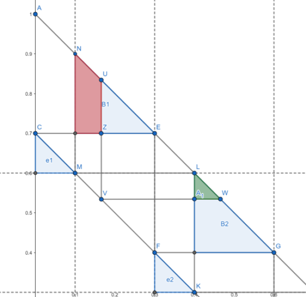
Nash Equilibrium

For any \(\mu_E \in \Omega^E\) \(\mu_B \in \Omega^B\) that satisfies above two properties, we have \((\mu_E, \mu_B)\) is a Nash Equilibrium.

No-Regret Learning

Learning algorithms always focus on two-part: exploitation and exploration. Exploitation indicates that to choose actions that have good performance in the past. Exploration indicates that to find potential good actions that have little chance to be played in the past.

Regret minimization learning algorithm updates the policy of actions. In brief, it can be described as a player who will choose an action more likely if this action has an overall better performance in history. The player does not need to make the action and see the payoff but just needs to make a fiction play and evaluate the outcome.

For an action profile \(a\in A\), let \(s_i\) be player’s (with player id \(i\)) action, and \(s_{-i}\) be all the other actions in this term. We denote the payoff as \(u(s_i, s_{-i})\). The regret algorithm will calculate the all the other possible actions \(s_{i'}\) with the payoff \(u(s_{i'}, s_{-i})\), and let the \textbf{regret} of not playing \(s_{i'}\) instead of \(s_i\) to be the expression \begin{equation} regret(s_{i’},s_{i},s_{-i}) = u(s_i, s_{-i}) - u(s_i, s_{-i}) \end{equation}

The regret will affect the future play in the following ways. The player will accumulate regrets for all the possible actions, and select the next action according to the previously accumulated regrets. To balance between the exploitation and the exploration, the player will choose the next action randomly according to the normalized positive accumulated regrets. This suggests that if an action has higher regrets, it will be chosen more likely. Notice that we have the following relation: \begin{equation} regret(s_{i’},s_{i},s_{-i}) = u(s_i, s_{-i}) - u(s_i, s_{-i}) = - regret(s_{i},s_{i’},s_{-i}) \end{equation}

This suggests that if the player chooses an action with high regret, the accumulated regret of other actions will be decreased. Therefore, this is the reason why the algorithm is named regret minimization, the player will tend to play with the least regret.

As a result of the Hart and Mas-Colell Theorem, if two players follow the regret learning algorithm, the empirical frequency of play converges to the correlated equilibrium set (CE set). Moreover, in the regret minimization algorithm, the regrets tend to be zero. Which is given strategies \((p^1,q^1),...,(p^{t-1},q^{t-1})\) there exists a strategy \(p^t\) and for whatever \(q^t\) is we have the following:

$$ \begin{equation} \left(\frac{1}{t} \sum_{s=1}^t u\left(e_i, q^s\right)-u\left(p^s, q^s\right)\right)_{i=1}^n \rightarrow C=\left\{a, a_i \leq 0 \right \} ; t \rightarrow \infty \end{equation} $$

Moreover, by Blackwall’s Approchability theorem, we have the distance between the CE set as \begin{equation} d(a_t,C) \in O(1/\sqrt{t}) \end{equation}

Learning Result

The learning shows a minimization of accumulated regrets. Also the action space converge to the CE set. As the learning to proceed, the average regret of both players keep decreasing in a sense of \(1/\sqrt{t}\).

In this section, we provide several simulation results for the cases \(E=0.3,0.6,0.7\). In each graph, the x-axis is the number of resources that Blotto put into Battlefield 1. Since we just consider the points on \(L_E, L_B\) we represent the regions of NE \(e_i,b_i\) by the interval on x coordinate.

From the previous analysis, we know that the NE are in \(e_1=(0,0.3), b_1=(0.3,0.7)\)

The NE are \(e_1=(0,0.2), b_1=(0.2,0.4)\) \(e_2=(0.4,0.6), b_2=(0.6,0.8)\)

The NE are \(e_1=(0,0.1), b_1=(0.1,0.3)\) \(e_2=(0.3,0.4), b_2=(0.4,0.6)\) \(e_3=(0.6,0.7), b_3=(0.7,0.9)\)

We can see that the action set of player2(green probability density distribution) converge to the \(e_i\) regions. The action of player1 (red pdf) converge to the \(b_i\) regions.

---
layout: page
read_time: true
show_date: true
title: "No-Regret Learning in Blotto Game"
date: 2022-08-20
img: posts/20220820/line8.png
tags: [dynamical system, machine learning]
category: project
author: Hanchun Wang
description: "How to learn from the failure?"
mathjax: yes
---